Lightweight Critical Path Analysis
TLDR
This feature performs a basic single rank critical path analysis. We demonstrated a walkthrough of using the tool.
Additionally, we dive into assumptions made and implementation principles.
Introduction
The key idea behind critical path analysis is to find operations in a large system that constitute the longest path between start and end. An operation on the critical path can significantly impact the program’s overall performance. In other words, reducing the duration of that operation will result in a measurable change in the overall timing This is illustrated in the figure below.
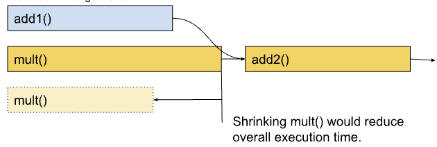
Critical paths can shift if an operator is optimized beyond a point; like the mult() in Figure 1 becomes shorter than add1().
Why?
Critical path analysis is a commonly applied technique in HPC and AI/ML optimization. It can be leveraged in two ways:
Performance/Efficiency opportunities: Operations/kernels on critical path should be the target of performance analysis and optimizations. They can provide the “best bang for the buck” for performance improvements
The critical path can give us a sense if the training iteration is X% CPU bound or Y% GPU bound, or Z% communication bound for distributed training.
The analysis is also not limited to just CPU/GPU kernels. Delays in launching or executing CUDA kernels can constitute a sizable portion of the critical path as well. This could be optimized by operator fusion (Pytorch2.0) and CUDA graphs etc.
Simulating Improvements/Gains: After identifying the critical path we can estimate improvements by simply modifying the graph and re-running the critical path finding algorithm.
Why Lightweight?
The space to build such kinds of analysis is vast. We could deduce the multi-rank critical path to better understand things like stragglers, and also consider tensor input/output dependencies among PyTorch operators.
To start with, we decided to simplify the dependency analysis between PyTorch operators. Our key core assumptions are.
All PyTorch CPU operators are dependent serially on the last operator that ran on the respective CPU thread.
In addition, we consider dependencies between CPU and GPU, both in terms of kernel launch, kernel-kernel delays and synchronization events.
The motivation behind this flavor of critical path analysis is to identify the primary bottleneck in the training loop - is it the CPU, or GPU compute or GPU communication.
The operator data-dependency part can be added later and further enable insights like re-ordering of operations and subgraphs. We can leverage Chakra Execution Traces to track data dependencies among tensors. This version of Critical Path Analysis does not need Execution Traces.
Using Critical Path Analysis
This ipython notebook illustrates basic critical path analysis.
Prerequisite
The PyTorch profiler traces were previously missing information regarding CUDA synchronization events. This was fixed in PR1 and PR2 . Follow the documentation here to enable CUDA synchronization events to get best results from this analysis.
Analysis:
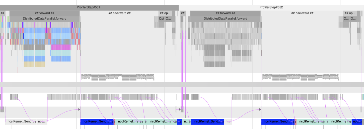
As shown in the notebook, use analyzer.critical_path_analysis() for trace events within a single rank.
We can further reduce the region of interest by selecting a trace annotation and instance id.
For example, you can use this to limit the analysis to one iteration by passing annotation ‘ProfilerStep#500’.
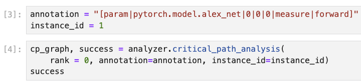
The output cp_graph object is a networkx.DiGraph object that is used as input for further analysis.
Visualizing Critical Path:
Now for the fun part.
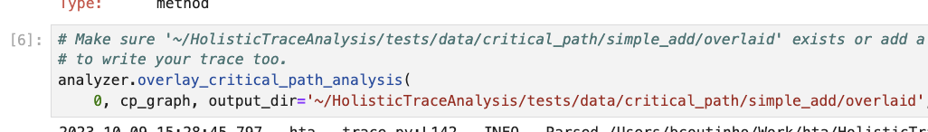
Use overlay_critical_path_analysis() function to visualize the critical path on the original trace file.
There are two modes for the output:
When
only_show_critical_events=True(default value) the output trace only contains CPU operators and GPU events on the critical path. One can compare it with the original trace to contrast the critical path identified by the algorithm.When
only_show_critical_events=Falsein the output trace file search for “critical” to highlight events on the critical path.
Edges in the critical path graph will be shown using arrows or flow events.
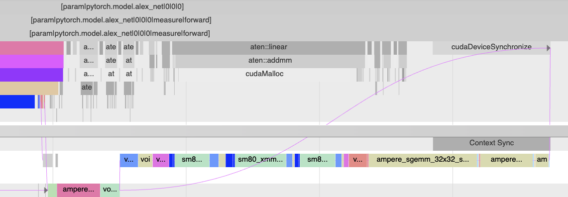
To illustrate this here is a simple training loop example on AlexNet, using setting (2) above. One can search for “critical” in chrome trace viewer to highlight the critical path. Most of the critical path is on the CPU here due to large delays in running cudaMalloc.
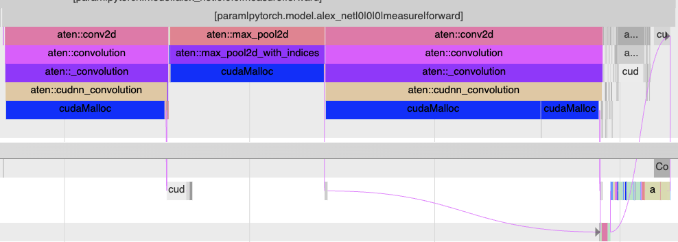
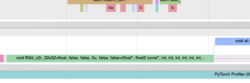
Zooming in to the right hand side, the GPU is now more busy and we can see the critical path flow from the CPU, to two different GPU streams and then up to the CPU again.
Unfortunately, the search based highlighting doesn’t work in Perfetto.
You can use the only_show_critical_events-True mode to display only the critical path events.
Large Training Job Traces
Here is an example of running this on an actual training job trace. In real life training jobs have pipelined stages so the we should run critical path analysis over two iterations. We can set the algorithm to run on two different iterations as shown below.
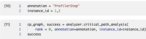
This analyzes the 2nd and 3rd iterations (551 and 552).
The critical path is initially on the CPU in step 551. Zooming in you will see many small GPU kernels, indicating that the GPU is not being kept busy. Increasing the batch size could be one optimization.
The critical path then shifts to NCCL all-to-all and all-reduce in the backward and next iteration forward pass. Thus communication imbalance is likely slowing down this workflow
Finally, on the tail end we see some GPU kernels launched by the optimizer on the critical path.
This workflow in general needs to better utilize GPU and fix NCCL imbalance issues.
Implementation Details
We drew inspiration from the previous work in academia to come up with our approach.
Design Overview
In a nutshell, computing the critical path involves 1) constructing a weighted DAG connecting all the operations, 2) finding the longest path in this DAG. The challenging part is constructing the DAG here.
Nodes: The Nodes in the critical path graph represent points in time. Each operator/kernel thus has two nodes viz. a begin and end node. In case of nested operators we also link the nodes in the order they appear in the call stack.
Edges in this DAG can be one of two types
Timing edges (weight = time): include durations for the operators/kernels as well as delays to launch operators between CPU and GPU.
Dependency edges (weight = 0): do not have a time component but show a dependency between operations themselves. This includes data dependencies and synchronization between CPU and GPU.
CPU Operator Nesting and Dependencies
Firstly, each operator gets a start and end node. To enable nested operators we basically add edges between start/end nodes of nested events. This is shown in the image below.
Since we are simplifying operator dependencies, each PyTorch top level operator has a dependency on the previous top level operator. More details in PR67
GPU Kernel Launches
CUDA is based on a highly asynchronous execution model for GPUs with up to 1024 outstanding GPU kernels at a time. To correctly determine how to connect GPU kernels and CPU operators we came up with two types of delays -
Kernel launch delays: There is a finite delay from kernel launch in the CUDA runtime to when the GPU kernel executes. This delay could either be due to the actual launch delay by system or the time spent waiting behind other kernels. We propose that kernel launch delay should only count if there are no outstanding kernels on a CUDA stream.
Kernel-Kernel delays: All GPU kernels on the same CUDA stream execute in order. Thus they have an implicit dependency on the previous kernel completing. We factor this into our DAG by adding “kernel-kernel” delay edges when there are more than 1 outstanding kernels on a CUDA stream.
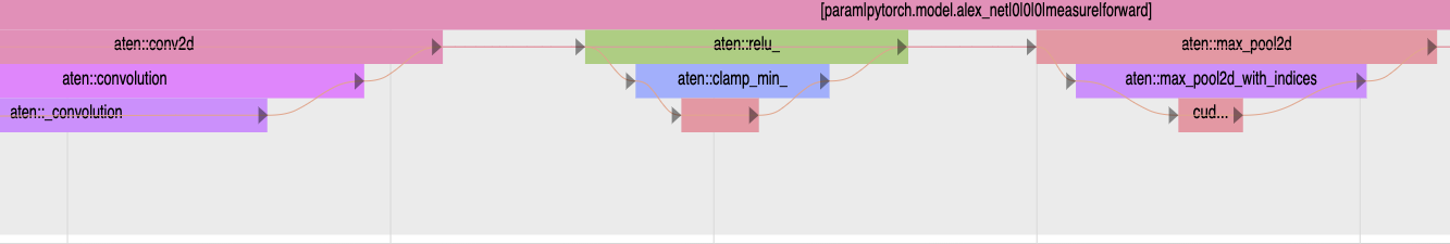
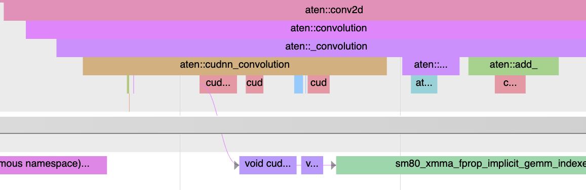
Here is an example of kernel launch and kernel-kernel delays in profiler trace (AlexNet). More details in PR68
Synchronization Dependencies
Lastly, the CPU will wait for the work dispatched to the GPU to complete. These are due to synchronization
Improving Profiler Traces: We realized the Kineto/PyTorch profiler was not providing enough information on Stream and Wait synchronization. To fix this we introduced CUDA Sync events in the trace. The new sync events can cover 3 kinds of synchronization we will describe below.
Synchronization Edges: Here is how we modified the DAG based on each synchronization type
Context / Device Synchronization: Since this is a global synchronization type we add edges from the last GPU kernel on all streams to the runtime function on the CPU calling Context/Device Synchronize.
Stream Synchronization: is similar to above but it synchronizes a single stream. Thus we only add a synchronization edge between the last GPU kernel on the specific stream and the corresponding Stream synchronization call on the CPU.
Event Synchronization: is a lot more complex and we explain it below. The above 1, and 2 cases lead to
GPU -> CPUsynchronization. Typically Event based synchronization is used forGPU -> GPUsynchronization.
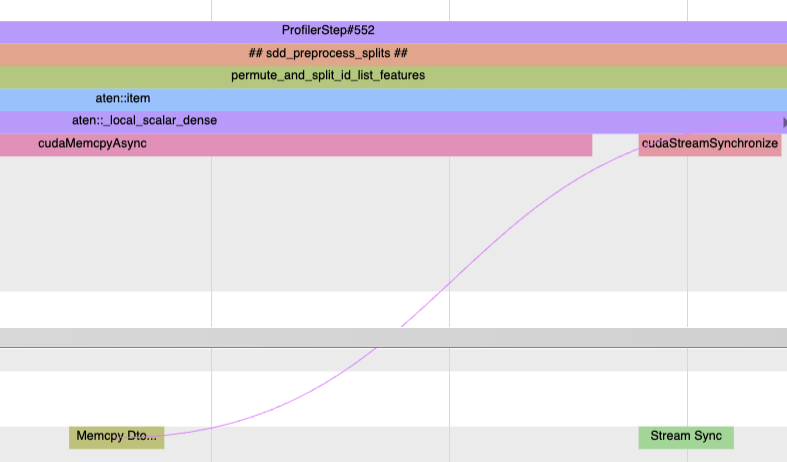
An example of CUDA Stream synchronization.
Handling CUDA Event Synchronization
In CUDA Event synchronization basically we have an event recorded on one stream and a GPU kernel waiting for that event to complete on another stream. Our approach is to trace this dependency
The newly added synchronization events
cudaStreamWaitEvent()informs us of when the event sync occurs, ID of the CUDA event and whichcudaEventRecord()is being synced on.The next kernel on the destination stream is the one that will wait.
We backtrack to the source
cudaEventRecord()function call on the CPU.Then find the preceding kernel launch and hence the kernel that ran on GPU due to it.
The two kernels in step (2) and (4) are the ones that need to be connected as shown in the figure below.
See PR69 for implementation details.
An example of Event synchronization aka inter GPU stream synchronization.
Future Work
Here are a few ways we can improve on this work.
Integrating Chakra Execution Traces - Chakra Execution Traces helps to add real CPU operator dependency edges and can surface opportunities with re-ordering of subgraphs for instance.
Summary Statistics: a natural extension of this work is to tabulate the time spent on CPU / GPU on the critical path with further details like time spent on kernel-launch delays, kernel-kernel delays and other overheads.
Simulating New Hardware and Optimization wins: the analyzer today does return a Networkx DiGraph object that one can modify and recompute the critical path. Additionally, it would be great to re-draw the trace and new critical path on the simulated optimizations or changes.